
Real-time PCR (qPCR) is the gold standard for measuring gene expression and detecting nucleic acids, but its results are only as good as its primers. Two quality checks decide whether qPCR data can be trusted: primer efficiency, which shows how well the target doubles each cycle, and melt curve analysis, which confirms that only the intended product was amplified.
This guide explains how to calculate qPCR primer efficiency, how to read a melt curve, and how to fix the most common problems.
What Is Primer Efficiency in qPCR?
Primer efficiency describes how close the reaction comes to perfectly doubling the target in every cycle. At 100% efficiency, the amount of product doubles each cycle. Lower efficiency means less product per cycle; apparent efficiency above 100% usually signals a problem.
Efficiency matters because the widely used ΔΔCt (delta delta Ct) method assumes that the target and reference genes amplify at close to 100% and at similar efficiencies. If they do not, fold-change results can be badly wrong.
How to Calculate Primer Efficiency
- Prepare a serial dilution of template (cDNA, DNA or plasmid), usually five to seven points in 5-fold or 10-fold steps.
- Run each dilution in triplicate with the primer pair.
- Plot Ct values (y-axis) against the log of template input (x-axis) to create a standard curve.
- Fit a straight line and note the slope and R² value.
- Calculate efficiency: E (%) = (10^(−1/slope) − 1) × 100.
Interpreting the Results
- Ideal slope: About −3.32, equal to 100% efficiency.
- Acceptable efficiency: 90–110%, corresponding to a slope of about −3.6 to −3.1.
- Linearity: R² of 0.98 or higher, ideally above 0.99.
- Matched efficiencies: Target and reference gene efficiencies should be similar for ΔΔCt analysis; otherwise use an efficiency-corrected method such as the Pfaffl method.
Why Efficiency Can Be Too Low or Too High
- Below 90%: Poor primer design, secondary structures, suboptimal annealing temperature, or low primer or magnesium concentration.
- Above 110%: PCR inhibitors in concentrated samples, primer dimers or non-specific products, pipetting errors, or including dilution points outside the linear range.
What Is Melt Curve Analysis?
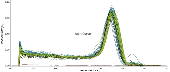
Melt curve analysis (also called dissociation curve analysis) is performed at the end of a SYBR Green qPCR run. The instrument slowly heats the products, typically from about 60–65 °C to 95 °C, while measuring fluorescence. As double-stranded DNA melts, SYBR Green is released and fluorescence drops.
The software plots the negative derivative of fluorescence (−dF/dT) against temperature. Each PCR product produces a peak at its melting temperature (Tm), which depends on its length and GC content.
How to Read a Melt Curve
- Single sharp peak: One specific product. This is the result you want.
- Extra peak at lower temperature: Usually primer dimers, which are short and melt at a lower Tm.
- Multiple peaks at higher temperatures: Non-specific amplification or genomic DNA contamination.
- Broad or shouldered peak: Possible mixed products; long or GC-rich amplicons can sometimes show complex melting from a single product.
- Peak in the no-template control (NTC): Primer dimers or contamination. A small primer-dimer peak in late-cycle NTCs is common but should be clearly separated from the target peak.
If the melt curve is ambiguous, confirm product size and specificity by agarose gel electrophoresis or sequencing.
qPCR Primer Design Tips for High Efficiency
- Primer length of about 18–24 bases with 40–60% GC content.
- Primer melting temperature around 58–62 °C, with the forward and reverse primers within about 2 °C of each other.
- Amplicon size of about 70–200 bp for efficient amplification.
- Avoid runs of four or more identical bases, hairpins and 3′ complementarity between primers.
- Span an exon–exon junction to avoid amplifying genomic DNA.
- Check specificity in silico with tools such as NCBI Primer-BLAST.
Optimising Your qPCR Assay
- Annealing temperature gradient: Find the temperature that gives the lowest Ct with a single clean melt peak.
- Primer concentration: Test a range of concentrations to reduce primer dimers while keeping sensitivity.
- Template quality: Check RNA purity and integrity, and use DNase treatment and no-RT controls.
- Controls: Always include NTCs, no-RT controls and validated reference genes.
Follow the MIQE Guidelines
The MIQE guidelines (Minimum Information for Publication of Quantitative Real-Time PCR Experiments) recommend reporting primer sequences, amplification efficiency, R², standard curve details and melt curve or specificity data. Following MIQE makes qPCR results reproducible and publication-ready.
Frequently Asked Questions
What is a good primer efficiency for qPCR?
Efficiency between 90% and 110%, with a standard curve slope of about −3.1 to −3.6 and R² of at least 0.98, is generally accepted.
How do you calculate qPCR efficiency?
Run a serial dilution, plot Ct against log input, and use the slope in the formula E = (10^(−1/slope) − 1) × 100.
What does a double peak in a melt curve mean?
Usually primer dimers or non-specific amplification. A lower-temperature peak typically indicates primer dimers.
Is melt curve analysis needed for TaqMan assays?
No. Melt curve analysis is used with intercalating dyes such as SYBR Green. Probe-based TaqMan assays get their specificity from the probe.
Conclusion
Primer efficiency and melt curve analysis are the foundation of reliable real-time PCR. Validating efficiency with a standard curve, confirming a single specific product with melt curve analysis, and designing primers carefully ensures accurate gene expression data that meets MIQE standards and stands up to peer review.